 arkana
The ZK Chronicles: Arithmetization
A look at the bridge between the representation layer of problems, and the proving layer.
Equipped with pretty much every primitive we’re gonna need for the rest of the road, and having gone through what zero knowledge truly means, we can finally explore how modern proving systems are actually built.
And as we’ve hinted a couple times throughout the series, the first step to this endeavor is to understand what treatment we should give to circuits (our chosen model for general, finite computation) in order to encode their information in a way we can use to craft our protocols.
There are multiple ways to go about this, but we’re just gonna be looking at the two most popular techniques, which should open the door to presenting some of the most pivotal proving mechanisms in the field.
This should be a fun one!
A Quick Recap on Circuits
Even though we’ve already talked about them extensively, it will be good for us to have a quick recap on circuits before we start.
Circuits are a general model for (finite) computation. At their core, they are just directed acyclic graphs where nodes represent operations (gates), and edges carry values between them.
When we think of circuits, the most common type that usually comes to mind is binary circuits, where gates operate on bits and perform operations like , , and . And while these are great for computers, they are not as convenient for the kind of algebraic manipulations required in most cryptographic protocols.
That’s the reason we explored how to translate these circuits into their finite field counterparts, by replacing boolean gates with field operations (addition and multiplication). The result of that process, which we called arithmetization, was a new kind of circuit called an arithmetic circuit.
For modern zero-knowledge systems though, this is barely the first step.
Arithmetization Revisited
When people talk about arithmetization in the context of modern proving systems, they usually mean something very different. And for our purposes, this second meaning will be much more important.
Our goal is no longer just to express a computation as an arithmetic circuit. Instead, we’re going to try and cast our circuits into a set of constraints.
What does this mean? Well, imagine we have an addition gate connecting wires with value , , and :
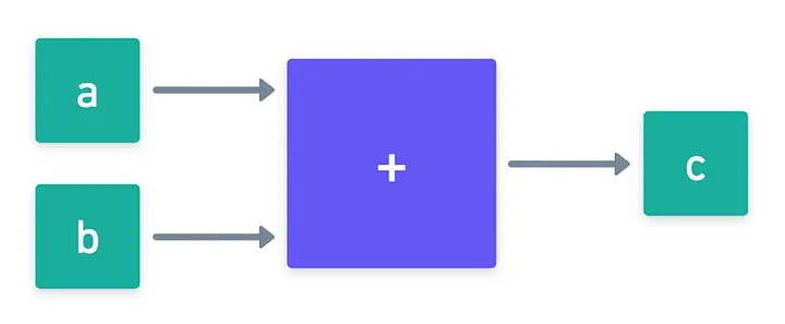
The trick is not just viewing this as a gate, but as a condition that must hold: must equal . If this is not the case, then these values cannot be part of a correct circuit evaluation. I know it sounds trivial to state this with such a simple example, but it’s an important conceptual reframing: we’re effectively defining a required relation between these values, otherwise known as a constraint!
There are many such types of relations we can establish between parts of a circuit, and depending on how we choose to do that, we’ll get a different set of constraints to represent the original circuit.
And so, from now on, whenever we speak of an arithmetization, it is this transformation from circuits to constraints that we’ll be referring to.
Great! But at this point, I guess you may be wondering why the hell you’d go through all this trouble!
A totally fair question. I don’t blame you.
The key here is that once we have these constraints, we can use them to write our circuits as polynomial relations. It’s a necessary intermediate step, but once we’re done with the full process, we can use these polynomials to apply very powerful techniques to verify those relations efficiently.
In fact, the result of these arithmetization processes is called an intermediate representation, a term that refers to any model of computation that’s suitable for direct application on an interactive proof.
Alright then! So how do these magic arithmetization techniques actually look like?
R1CS
We’ll start with one of the most widely used constraint systems in ZK: Rank-1 Constraint Systems, or R1CS for short.
Quite a weird name, huh? We’ll see where this comes from further ahead!
To understand how this works, we'll first need a circuit to work with. Take for example this little guy over here:
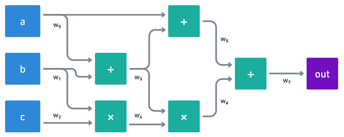
As you can see, we begin by labeling the connections just like in the image above. One key observation there is that branching outputs (or circuit inputs) share the same label, and this makes sense because they really share the same value.
And while that seems quite obvious, we'll later see that it's not always an easy condition to enforce!
Cool, so then, let’s think about what happens when we evaluate the circuit. A typical evaluation starts by providing values for the inputs , , and , and then by traversing the graph, filling in the values for the wires . Once we’ve finished, we'll get a new picture where all the wires will have an assigned value.
Which means that, if we write those wires in order, we end up with an evaluation vector containing the resulting wire values:
Nothing too special, right? Obtaining a vector of the like is as easy as evaluating the circuit. But if we flip the question around, this vector gains a whole new meaning:
Does any vector correspond to a valid circuit execution?
Clearly, the answer is a resounding no: we know some relations must hold between some of the vector’s coordinates. So a vector that satisfies all these relations corresponds to a valid circuit evaluation, and we call it a witness.
Which should ring a bell, right? Yeah, it sounds like our language and witnesses framing!
Recall that a language is just a set of valid statements, and a witness is the extra information that proves membership in that language.
Here, our language is the set of all valid circuit evaluations, and is exactly the witness we’re looking for: the full record proving that a circuit was evaluated correctly.
There's one subtlety worth noting here, before we even put any arithmetization to use: the statement is public, while the witness is private. In other words, the circuit itself (plus any public inputs and outputs) is known by all parties, but the full evaluation, including secret inputs and intermediate values, is known only to the prover!
This distinction will matter a lot more when we get to the actual proving systems that use the techniques we’re presenting today, but it’s good to have it in the back of our minds for the time being!
In short, the prover holds , and the verifier doesn’t. And so, what we need to capture is how to identify whether a witness is valid, because that’s precisely what will determine whether evaluation is correct or not.
And that's exactly what R1CS tries to capture.
The Constraints
I guess the easiest way around this will be to go gate by gate through our circuit, and write down what must hold for each one of those gates. Here’s the image again, so you don’t have to scroll back up:
We’ve got a total of five gates in there, three for addition and two for multiplication. Each of the gates involves only three of the wires, so in order to use our witness to represent these relations, what we want to do is to somehow pick and choose which wire interacts with which.
This can be very elegantly done using what we call a selector vector, and the idea of an inner product we looked at a couple articles back:
Inner products behave very nicely for addition, and in fact, we can use them to condense multiple successive additions. For example, we can coalesce the two gates at the top into a single inner product:
Though we may or may not do this in practice, it’s definitely a possibility.
Multiplication gates are not so well-behaved though. They present somewhat of a challenge in terms of their inner product representations, because as long as the selector vectors only holds integers, all we can get is a linear combination of the coordinates of . The simplest way to represent a multiplication then is to actually multiply two inner products together, like this:
And believe it or not (and almost by accident), we have actually arrived at a form that allows us to represent all relations in the circuit!
For example, take the second multiplication gate. You can check that vectors , , and are the exact representation of the relation established in the gate!
The idea behind R1CS is that we can represent the whole circuit as a list of such vector triples (, , ), one for each gate. Not only that, but we can also nicely stack them into matrices, with one of these vectors per row, making it so that our entire circuit can be fully described as three matrices , , and , and we can just write the whole system as:
And here, we can shed some light on the naming: the row constraints are what we call rank-1 conditions.
Each of the inner products in the left-hand side of that expression results in a scalar (a single finite field element in our case), and we can always write the product of two scalars as what’s called a quadratic form. This is, we can work the product into the form , where is a rank-1 matrix, since it’s the outer product of two vectors.
Stack of these conditions together, and you get a Rank-1 Constraint System!
Clean, eh?

Quick clarification: the symbol in there denotes entry-wise product, also called the Hadamard product.
Any valid circuit evaluation will have to satisfy that equation above. Which means that we’ve effectively moved from a CSAT problem to an equivalent R1CS-SAT problem.
Great! We have our new, shiny representation. But checking that satisfies the R1CS system is not necessarily a simple task... and can we even do it efficiently?
Encoding
We’ve actually already hinted at what’s coming next a couple times, so you might expect it by now: we encode everything into a polynomial identity!
It might sound a little scary, but in this case, it's actually a surprisingly simple process. There’s a total of constraints to encode (one for each gate, or per matrix row), so what we’re gonna do is take each column of our matrix (which represents all the selectors for a single wire), and interpolate a polynomial that passes through its values.
And as you already know, we use the th-roots of unity () as indexes so we can do this efficiently thanks to the Fast Fourier Transform, where is the number of constraints, or gates, or matrix rows.
We’ll do this for each matrix, giving us a total of three polynomials for each wire, which we’ll denote , , and . Note that when we evaluate, say, , what we’ll get is the element in the matrix at row and column .
I know the row and column index convention is usually the other way around, so I hope this is not terribly confusing! It's just how it's stated in most literature, so blame the people that came before me!
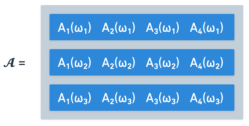
For any single row, what we have are all the selectors for the witness vector, and the value simply allows us to choose which row we’re looking at. And focusing on a single row, we can define this polynomial right here, which corresponds to the inner product between the witness and the selectors of row :
We can do just about the same with the other matrices - and knowing that the constraint at each gate can be represented as a product of inner products, we can directly translate this into a relation between some evaluations of our encoded polynomials:
Furthermore, we can rewrite that relation as:
Which means (drum roll, please) that the polynomial happens to have roots at these roots of unity! And this is huge: it means we can perfectly divide that expression by this other polynomial here, which we call a vanishing polynomial:
Because it vanishes (evaluates to ) at a set, in this case the th-roots of unity.
So the final step is to write the following relation, for some quotient polynomial :
This is what’s called Quadratic Arithmetic Program (QAP) relation.
Quadratic because the core relation is a product of two polynomials, arithmetic because we’re working over a finite field, and program because it encodes a computation. Simple as that!
Crucially, we see that a witness satisfies the R1CS relation if and only if that polynomial identity right there holds. So, in essence, we’ve condensed all the constraints into a single polynomial identity! Isn’t that neat?

From here, what we need to do is craft some proving mechanism for a prover to convince a verifier that this relation holds. That means we’ve only gotten halfway through solving the problem, but this is exactly what we set out for: a representation that proving systems can work with.
While the math works, R1CS has some practical shortcomings that are worth acknowledging before moving on.
Perhaps most obvious is the fact that those matrices will become quite large really fast as the circuit size grows. Plus, the vast majority of matrix elements will be zeroes (each constraint involves only a handful of wires), so we’re dealing with sparse matrices. That means that for large circuits, we’re packing a large amount of nothing into our polynomial encodings, which is rather inefficient.
There’s also a rigidity problem: we can only encode one product per constraint. Anything more complex than that must be decomposed into simpler constraints, which further enlarges the matrices.
And so, to mitigate these problems, other arithmetization techniques have emerged over time. One such evolution is the one we’ll be focusing on next.
Plonkish
The weird name of this next arithmetization comes from the paper that first introduced it, and the argument system it described: Permutations over Lagrange-bases for Oecumenical Noninteractive arguments of Knowledge - or PLONK, for short.

Yeah, don’t worry too much about the naming. We’ll look at that in due time!
What’s important here is that the arithmetization technique happened to transcend the particular argument system, having seen application in other protocols. So it has gained a name of its own: Plonkish.
In order to more efficiently represent the circuit’s constraints, Plonkish takes a different approach from R1CS, and places the focus on each gate. You see, every gate involves just a handful of wires, so the proposition here is to only encode those, and avoid involving the rest of the circuit.
Sounds promising, right? But how do we do that?
The Table Approach
The core idea behind Plonkish is to throw the matrix representation out the window entirely, and instead organize the circuit as a different construction: a table. Each row in said table corresponds to a gate, and we have (at least) three columns for the wire values involved: a left input , a right input , and an output . For our example circuit:
Said table would look something like this:
| Gate # | Left input | Right input | Output |
|---|---|---|---|
| 1 | |||
| 2 | |||
| 3 | |||
| 4 | |||
| 5 |
That’s much, much more dense right off the bat, right? So it seems we’re starting on the right foot!
This table is usually called the execution trace of the circuit. Sure, it's really simple... but it’s also clearly missing one important thing: the gate types. In other words, how do know just by looking at this to expect to equal , and not ?
And that’s where the real magic of Plonkish resides: we can expand the above table with some extra columns, that add all the necessary data to determine what kind of relation to check.
We can actually take it one step further, and define a couple more knobs, also called selectors:
These new parameters are flexible enough for us to represent any single gate, namely:
- For an addition gate, we’d set , , and , while the other values would be set to .
- A multiplication gate would require , and .
- We could even represent a constant gate, setting , and for example .
With just this little template expression, we have all the expressivity we need to represent an entire circuit, wasting much less space than in our previous effort.
And we don’t have to limit ourselves to these selectors either: some systems define custom selectors for added efficiency. Notable examples are Plookup introducing lookup tables (we'll look at this later), TurboPlonk adding custom gates, and UltraPlonk being the lovechild of both techniques.
Copy Constraints
Everything sounds great so far: smaller tables, simple selectors... it’s almost too good to be true, isn’t it?

Yup. There is a problem, and a pretty big one at that.
Let’s look at that table from before one more time:
| Gate # | Left input | Right input | Output |
|---|---|---|---|
| 1 | |||
| 2 | |||
| 3 | |||
| 4 | |||
| 5 |
As you can see, appears a total of three times. It’s clear that every instance of should have the same value, but when we look at an evaluation trace, there’s nothing enforcing that condition. In other words, individual rows can be correct, but we need some way to encode that those instances of should all have the same value.
Notice that we didn’t have this problem in R1CS, as the witness vector had a single entry for , so consistency was guaranteed by construction. That’s not the case here!
This is what we call a copy constraint, and enforcement happens through a permutation argument (hence PLONK’s weird name). Nevertheless, that’s the job of PLONK, and is not an intrinsic characteristic of the arithmetization itself. We’ll look at that when the time comes, so just keep that in mind for now!
And there you have it! That’s the intermediate representation we’re after.
Of course, the next step will be to take that table and, in similar fashion to R1CS, encode it as a polynomial over the roots of unity, one evaluation per row.
The result is a rich and structured polynomial representation of the entire circuit, which gets even richer once we include the polynomials required for the permutation argument (hint, hint). It’s dense, flexible, and perfect for modern proving systems, and that’s the main reason it has outlived its original environment, and is applied in modern ZK systems like Halo2.
Summary
That’s a wrap on arithmetization!
At least for now!
It might not seem like it, but what we've accomplished today is huge: we’ve turned a question about correct circuit evaluation, into algebra that a proving system can work with and reason about.
Or put in other words:
We now have the bridge between computation and algebra that modern proving systems are built upon
Sure, the details are different, but the end goal is much the same. Choosing the right arithmetization technique will depend on a blend of efficiency, convenience, and security, making it so that there exist protocols using either of the two methods we described today, and even other methods we're yet to describe.
Speaking of which, we have just about everything we need to put R1CS to good use, by looking at one of the most influential proving systems ever designed. It’s compact, fast to verify, and built almost entirely on the QAP relation we derived today.
Hope that’s enough to keep you hooked! I’ll see you on the next one!
Did you find this content useful?
Support Frank Mangone by sending a coffee. All proceeds go directly to the author.